Introduction to Mitsubishi GX Works2 Ladder Logic Programming

Introduction

Every PLC software has its syntax for programming its brands of PLCs. As an engineer or technician interested in building a career in Controls, learning the programming syntax of each OEM is essential. Programming a Mitsubishi PLC is not as complicated as you might think, as it shares a common syntax with other PLC brands like Siemens.

In this tutorial, you’ll learn how to program basic ladder logic instructions for a Mitsubishi PLC in GX Works2.

Prerequisite

To follow along with this tutorial, you will need the following:

• An understanding of Mitsubishi GX Works2.
• An installation of GXWorks2

Bit Logic Instructions

Bit instructions are instructions that are usually the basics of PLC programming. These instructions can be found at the top right corner of the GX Works2 programming software Toolbar, as seen in the images below.

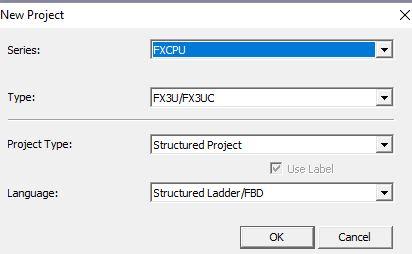
Launch the GX Works2 Software and configure your project as shown below

The instructions there are listed below from left to right;

• Open contact: This is also known as a Normally Open contact, which goes true when a signal is applied. This is especially used in the latching of coils.
• Close contact: This is also called a normally closed contact that goes false when a signal is applied.
• Open branch: This is used to create an alternate branch with an open contact in the same network.
• Close branch: This is used to close the alternate branch with a close contact.
• Vertical line segment: This is used to create a vertical line in the case of alternate branching
• Horizontal line segment: This is used to create a horizontal line in the case of alternate branching
• Coil: This is an output instruction usually at the end of a network. Its state is dependent on the conditions before it.

To use the branch instructions, select the open branch and place the cursor at the particular point on the network you want, as shown below.

• Element selection window: This window brings out the toolbar that contains all system functions and function blocks that can be used in programming.
• Input label: This label provides tagging options to instructions as input devices.
• Output label: This label provides tagging options to instructions as output devices.
• Rising pulse: This is an open contact that goes only true when the input signal state changes from 0 to 1 at every positive trigger.
• Falling pulse: This is an open contact that goes only true when the input signal state changes from 1 to 0 at every positive trigger.
• Rising pulse close: This is a  close contact that goes only true when the input signal state changes from 0 to 1 at every positive trigger
• Falling pulse close: This is a close contact that goes only true when the input signal state changes from 1 to 0 at every positive trigger.

Control scenario

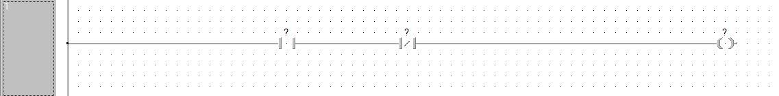
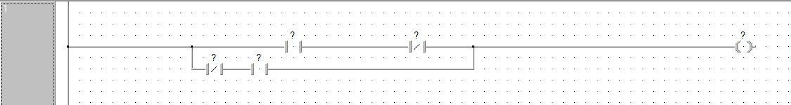
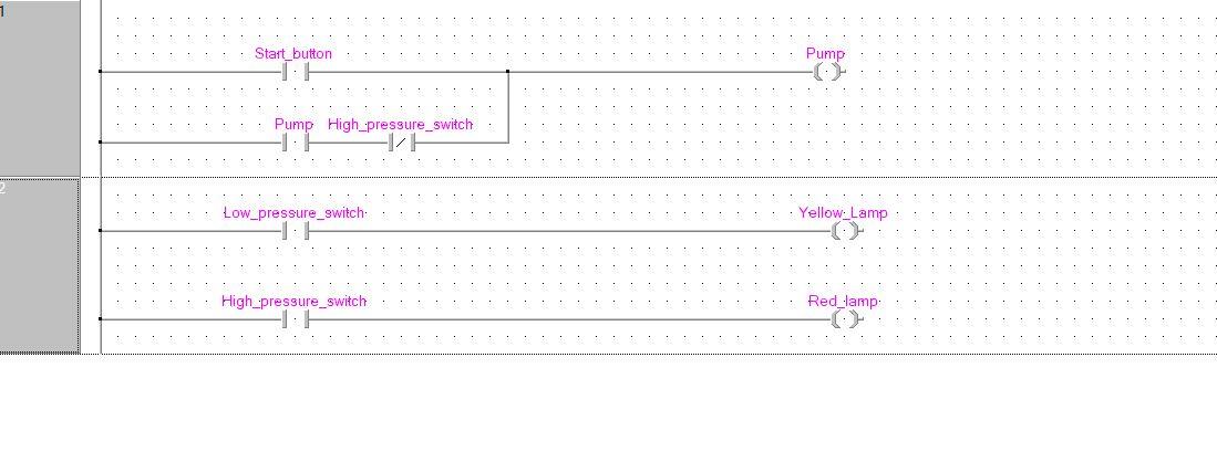
We will maintain the pressure in a receiver on a compressor application. Two pressure switches activate at 50 bar and 120 bar (low and high). To control the pressure, we have one pump. We want a red indicator lamp to be active when the high-pressure switch is active and a yellow indicator lamp when the low-pressure switch is active.

When we press the start push button, the pump should start immediately. Then, the pump turns off when the high-pressure switch is active only.

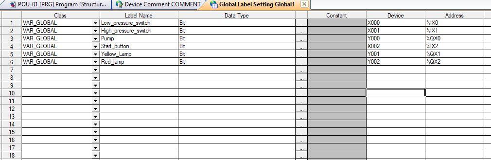
IO Addresses

Low pressure switch:  X000 

High pressure switch:  X001

Pump: Y000

Start button: X002

Red Indicator: Y001

Yellow Indicator: Y002

Testing

Create the tags by navigating to Global label. The window should look like the image below

Input the different Io devices as shown below

The tag pops out in the programming window (POU_01) by typing the label name. Program the control scenario as seen below.

Compile and rebuild all. Under the Program setting, call the program (POU_01) in the execution program. Every new program section must be called under the execution program; otherwise, the CPU won’t load it. 

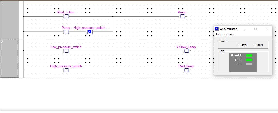
The first program will be called automatically by default. You can then start the simulator and run.

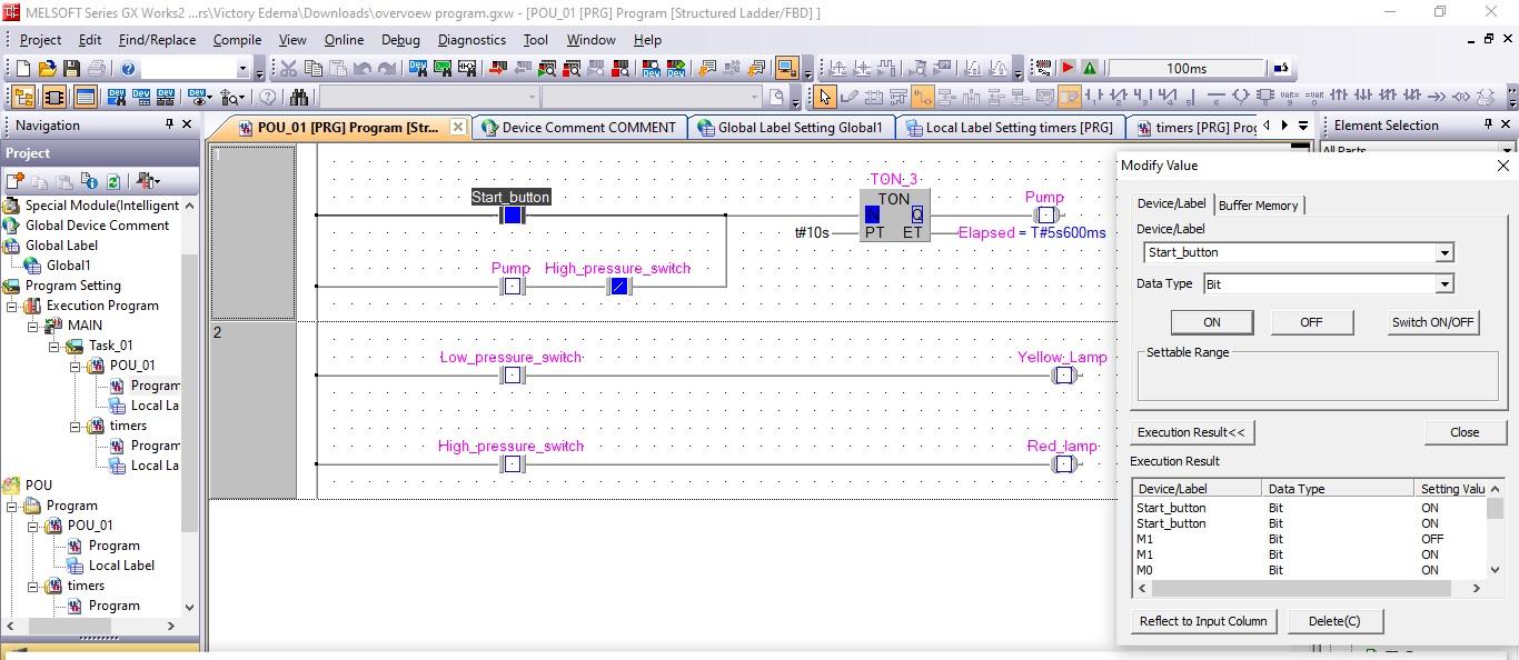
In the first network, the start push button energizes the pump. The start push button is latched because a push button is momentarily on the circuit. It is interlocked with the high-pressure switch.

In network 2, the low-pressure switch energizes the yellow lamp, and the high-pressure switch energizes the red light.

Right-clicking on a contact will bring out the options to modify the signal, or you can access it by double-clicking on the contact.

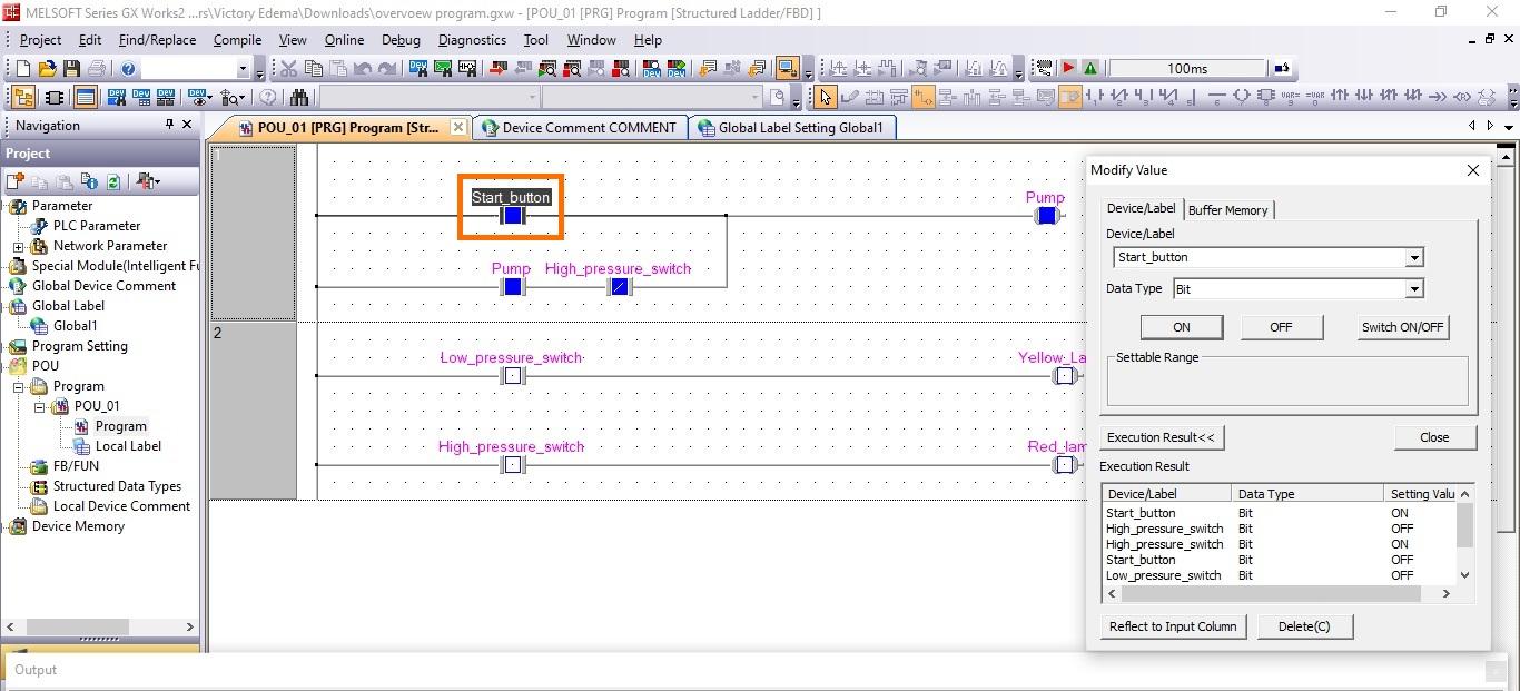
Make sure to test out the different criteria.

Timer Instructions

Like most programmable logic controllers in the market, Mitsubishi has its versions of timers. These are similar but not necessarily set up the same as the other manufacturers.

There are two commonly used timers Time ON timers (TON) and Time OFF timers (TOF). 

There are versions (Data Types) of the timer functions that have an added EN (enable) added to the input to control when the Time starts to lapse. These functions usually have an "_E" in the name of the function definition (TON_E). 

To add the timer function to your program,

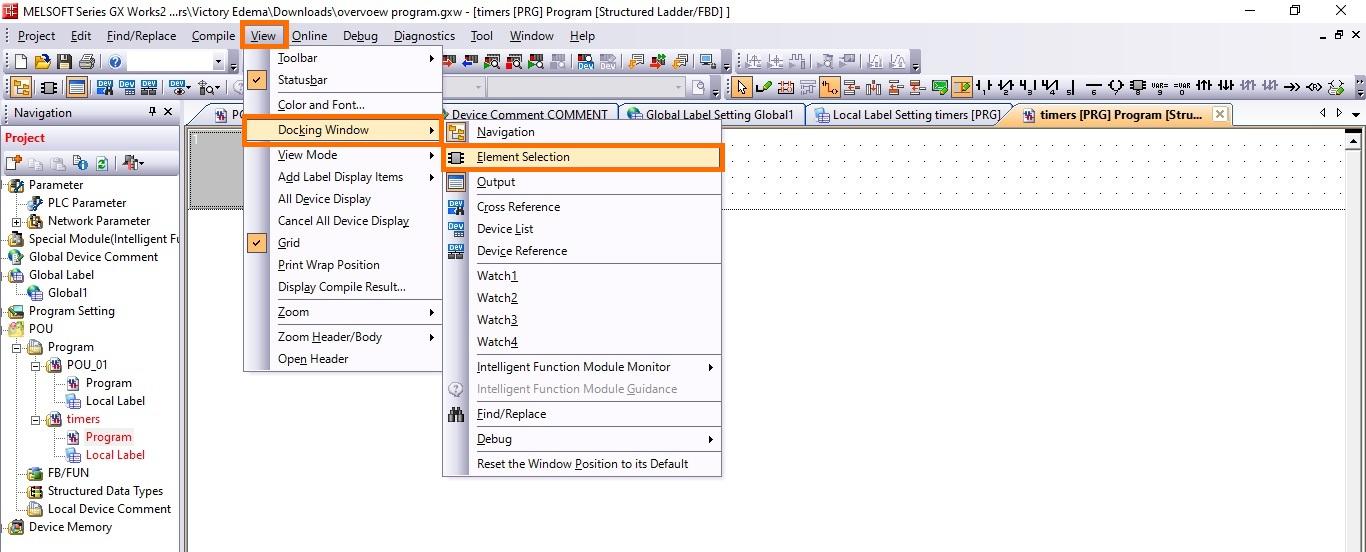
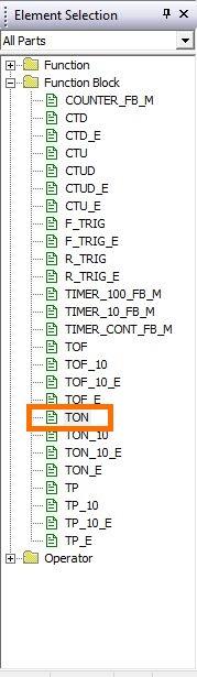
You can start typing TON or TOF or drag and drop the POU (function) from the element selection bar, usually on the editor's right. If the element selection window is not active, you can access it by navigating to the view and then the docking window. The timer will be located under function blocks.

Timer ON

By dragging the TON timer into your program, a window pops out. The TON gives an output when the ET value equals the PT value. It is a delay ON timer.

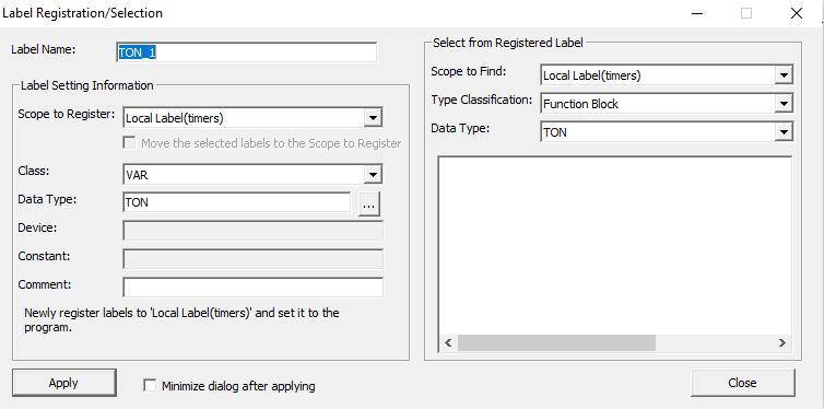
Label name: This is the name of the timer

Scope to register: Local scope means the timer can only be controlled and accessed from this program. Global means the timer can be accessed from anywhere in the program.

Class: VAR indicates a variable you can control, while VAR_CONSTANT means you are giving the timer a fixed value.

The PT input is a TIME data type. This is important to remember.  With Timers, you start with a “T#” followed by the time of preset you wish to use.  After the time, you will need to designate whether the time is in seconds (S) or milliseconds (ms).

The ET is for elapsed time.

Timer OFF

The TOFF is the opposite of TON. The output goes off when the PT value is reached. It is a delay off-timer.

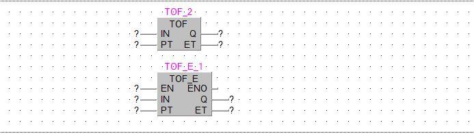
A Timer pulse (TP) gives an output while the ET value is yet to equal the PT value.

Control scenario

Using the same previous control scenario, make the pump come on after 10secs.

Data Move Instructions

The PLC uses data registers to store measurements, output values, intermediate operation results, and table values. The math instructions on the controller can read their operands straight from the data registers and, if desired, write their results back into the registers. However, these instructions also enable additional " move " instructions, allowing you to copy data across registers and write constant values to data registers.

Moving individual values with the MOVE instruction

The MOV instruction “moves” data from the specified source to the specified destination.

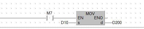
1) Data source (this can also be a constant). The "s" in Ladder Diagram instructions means source.

2) Data destination (In Ladder Diagram instructions, "d" means destination. In the example, the value in data register D10 will be copied to register D200 when input M7 is on. 

Pulse-triggered execution of the MOV instruction

Sometimes, writing the value to the destination only once within a program cycle is preferable. For instance, you would wish to do this if other program instructions also write to the same goal or if the transfer operation needs to be completed at a specific time.

The MOV instruction (MOVP) will only be performed once if a "P" is added to it on the rising edge of the signal pulse produced by the input condition. In the example below, when the state of M10 switches from "0" to "1," the contents of D100 are written to data register D200.

Moving 32-bit data

To move 32-bit data, just prefix a D to the MOV instruction (DMOV):

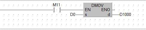
When M11 switches from “0” to “1”, the contents in D0 and D1 are copied into D1000.

There is also a pulse-triggered version of DMOV, DMOVP, which copies the 32-bit data at every rising pulse.

Moving blocks of data with the BMOV instruction

Only single 16-bit or 32-bit values can be written to a destination using the MOV instruction previously explained. To transfer consecutive data blocks, you can program several MOV instruction sequences. The BMOV (Block Move) instruction, offered mainly for this purpose, is more effective.

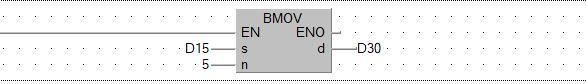
• S: Data source (16-bit device, first device in source range)
• D: Data destination (16-bit device, first device in destination range)
• N: Number of elements to be moved

In the above example, the contents in D15,D16,D17,D18,D19 will be transferred into D30,D31,D32,D33,D34 because the number of elements is 5.

BMOV also has a pulse-triggered version, BMOVP.

Comparison instructions

Comparison instructions are used to compare two values together. There are so many of these instructions. Amongst which are 

• Greater than (GT_E) : This outputs true if the value of IN1 is greater than IN2
• Greater down or Equal to (GE_E): This outputs true if the value of IN1 is greater than or equal to IN2
• Less than (LT_E): This outputs true if the value of IN1 is less than IN2
• Less than or equal to (LE_E): This outputs true if the value of IN1 is less or equal to IN2
• Not equal to (NE_E): This outputs true if the value of IN1 is not equal to IN2
• Equal to (EQ_E); This outputs true if the value of IN1 is equal to IN2

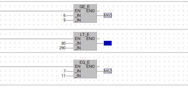
We can see that only the LT_E instruction gives an output because that is the only instruction that satisfies the condition. 

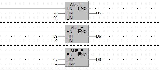
Math Instructions

In the element selection window, under operator, there are various math-related operators such as

ADD, MUL, DIV, SUB. As the name implies, they perform the same way a typical math operator works.

Conclusion

In this tutorial, you learned the basics of ladder logic instructions for programming a Mitsubishi PLC in GX Works2. You can learn about the other instructions not covered in this tutorial by going to the help file under the Help toolbar.