An Introduction to Servo Motor Programming in Siemens TIA Portal

Introduction
Today, there is very little chance that you will come across an automatic industrial installation without servo motors. these are essential components of modern industry and can be found in most applications.
A servo motor is a regulated motor (usually a brushless motor coupled with an incremental encoder) capable of performing high precision positioning and controlled by a drive.
In this tutorial, we will see how to perform simple positioning applications in the Siemens TIA Portal environment. Thanks to Siemens’ Technology Objects, configuring and programming servo drives has never been easier. The PLC is connected to the servo drive through PROFINET and we are assuming that the electrical parameters of the drive have been properly set.
Prerequisites
To follow along with this tutorial, you will need an installation of TIA Portal and Startdrive.
We will be using TIA Portal and Startdrive v17; other versions of software packages may also be compatible with this tutorial.
Configuring a servo drive in TIA Portal
Let’s begin by creating a TIA Portal project. You can choose any CPU supporting PROFINET. In this case, we’ll use a simple S7-1200C with its IP address kept at the default value {192.168.0.1/255.255.255.0}.
Then, we have to add the servo drive to the project. Click on “Add new device” in the project tree.
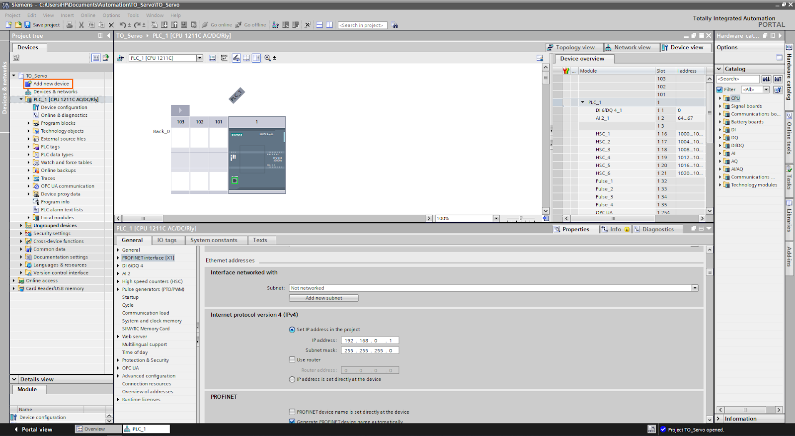
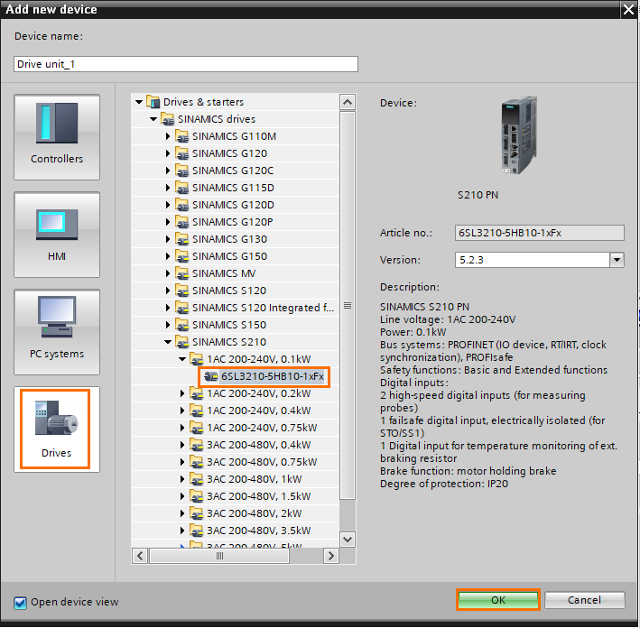
A small window containing the catalog of all devices available in your software will appear.
Open the SIMATIC S210 folder and select the model that suits your requirements. For this tutorial, we’ll use the simplest model of S210 (1 AC 240V, 0.1kW).
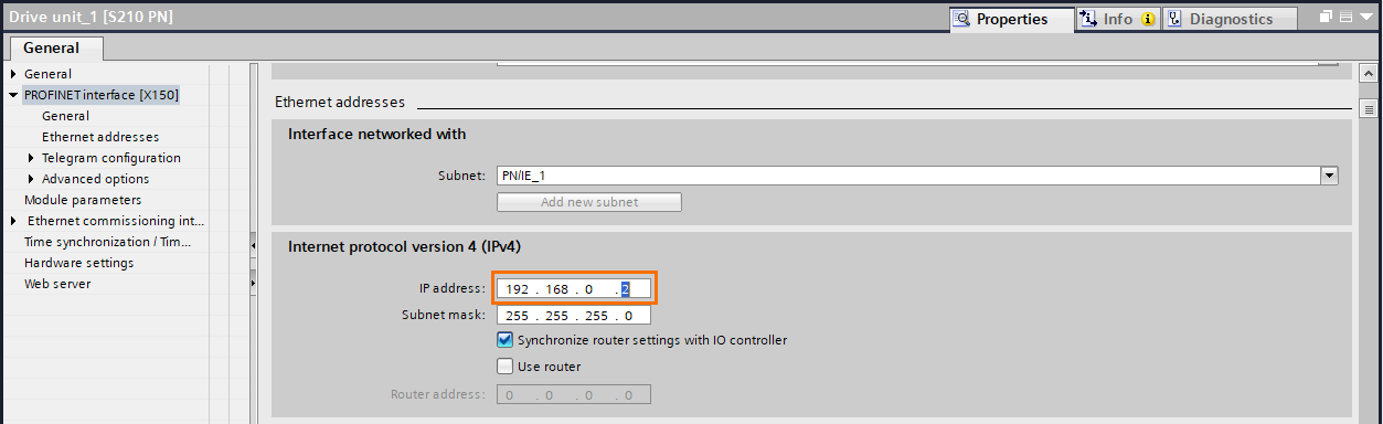
Now on the device’s properties view, click on “Add new subnet” to create a new network that we’ll link to the CPU.
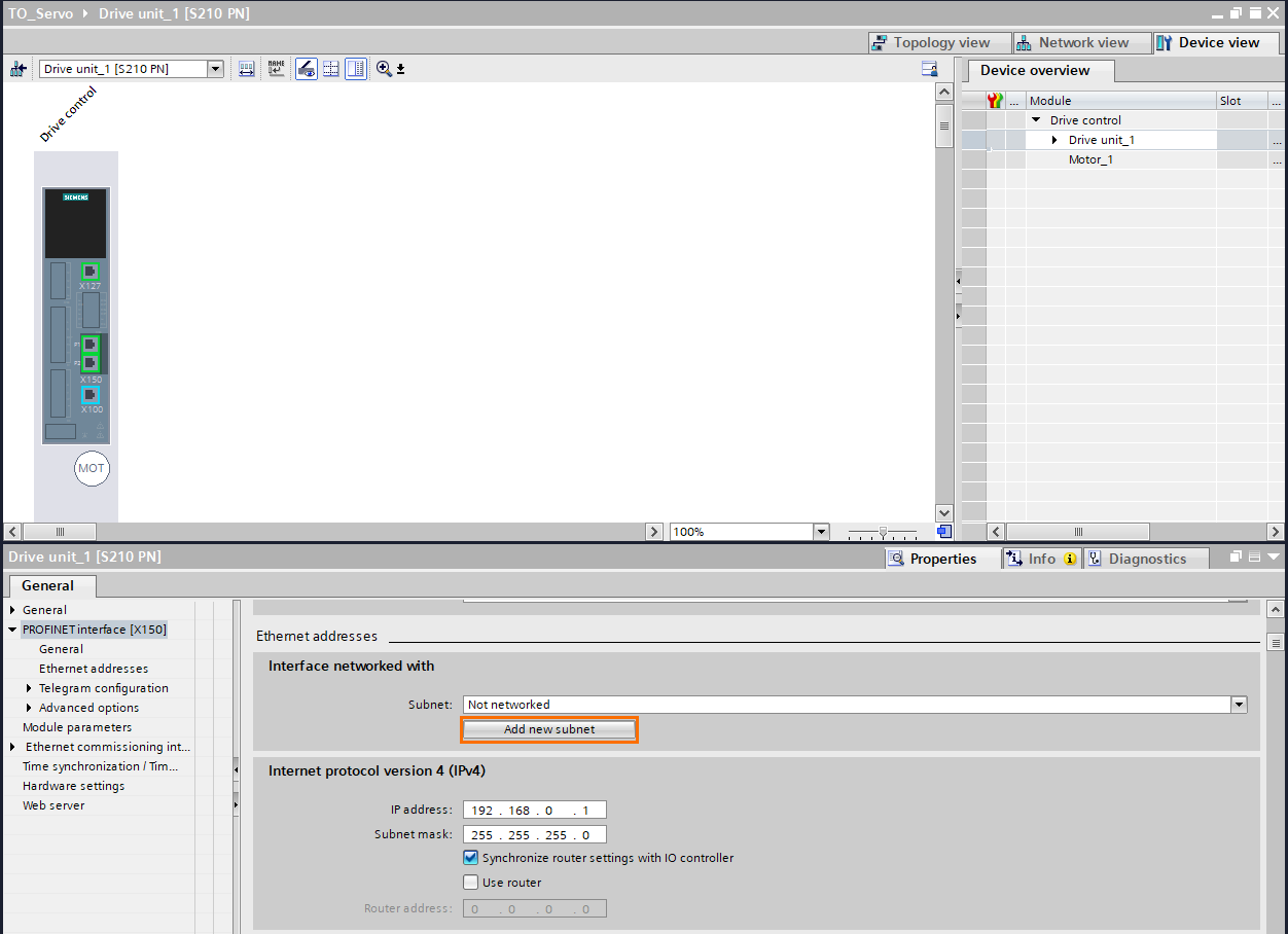
After that, edit the IP address f the drive so that it won’t conflict with the CPU address.
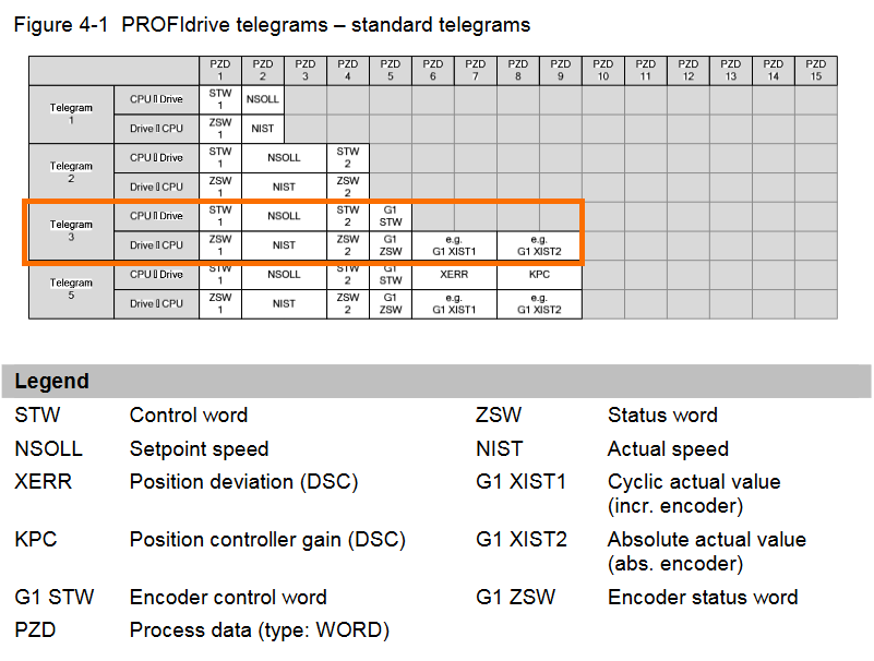
Next, we need to define the type of messages we want to communicate with the drive. These come as standardized messages (or Data blocks) called Telegrams. Each type contains a certain number of data with different lengths.
According to the official documentation, to have access to the encoder position value, we have to use telegram 3 or higher.
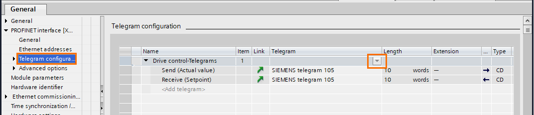
On the left side of the parameters screen, click on “Telegram configuration. You’ll find that the default telegram is set at “SIEMENS telegram 105” which is exclusive to the Simatic drives. To access any servo drive, we have to use a “Standard telegrams”
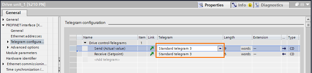
Click on the scroll on the telegram section and select “Standard telegram 3’ This will allow us to have access to Control words, Setpoint speed, actual speed, and the encoder values.
You can find the data addresses affected in the CPU by the telegram in the network configuration. You can edit the addresses to any memory area you desire. These values have been kept at their default values.
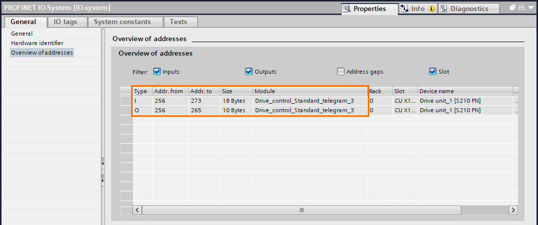
For this example, the data are addressed as follows:
- IW256: ZSW 1
- ID258: NIST
- IW262: ZSW 2
- IW264: G1 ZSW
- ID266: G1 XIST1
- ID270: G1 WIST2
- QW256: STW 1
- QD258: NSOLL
- QW262: STW 2
- QW264: G1 STW
In the absolute, you can perfectly control the servo drive by directly reading and writing the addresses in your program. But as you will see later in this tutorial, there’s a way more efficient tool that will allow us to pilot the servo motor more easily and clearly.
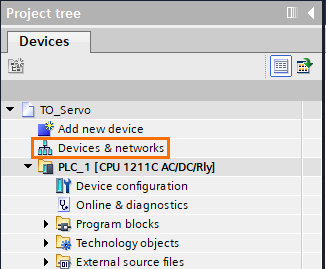
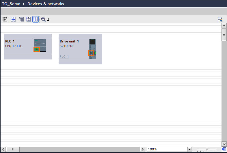
Next, we have to properly configure the communication between the drive and CPU. Click on “Devices and networks” in the Project tree.
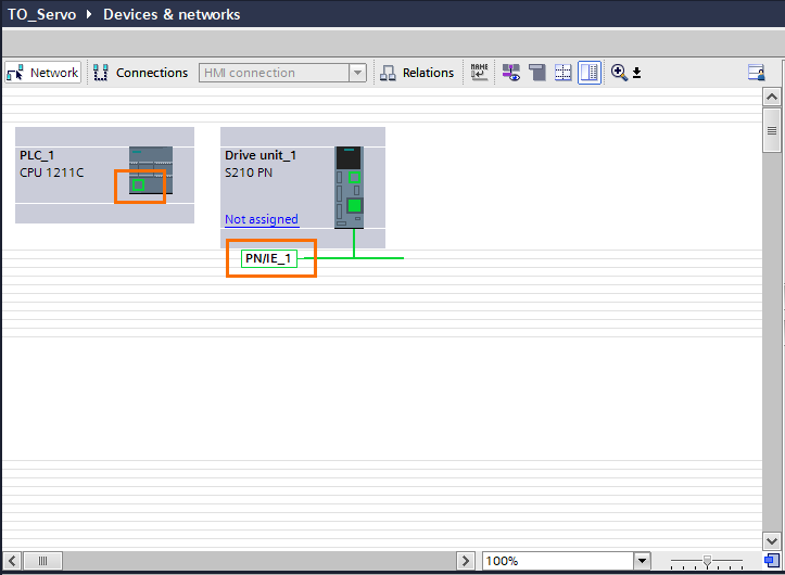
You can notice that the CPU is not connected to the PN/IE_1 network. Click on the green port on the CPU and drag it to the PN/IE_1 line.
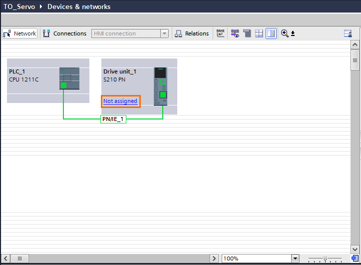
Now we have to tell the drave that he’ll have to talk to this CPU. Click on the CPU's green port PLC_1 as the main partner.
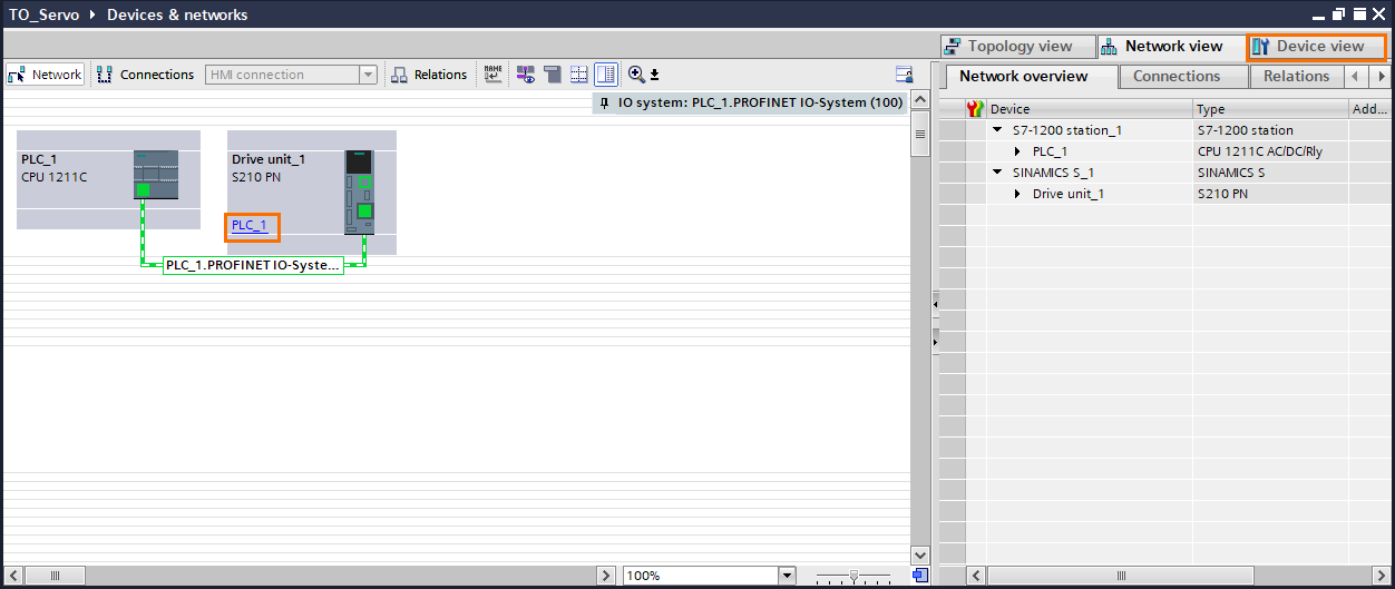
For the next part, we need to specify the actual physical ports used. Click on “Topology view”
As you can see, the two devices are not physically connected. Click on the port on the CPU and drag it to one of the ports of the drive.
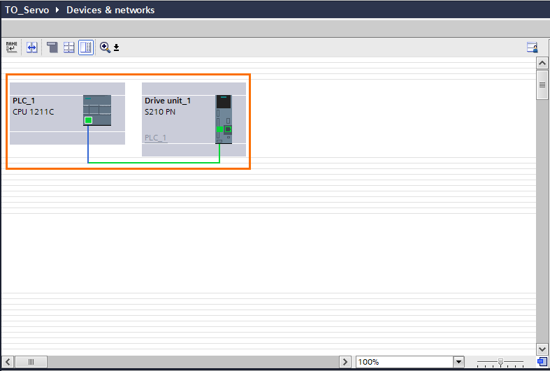
Now that all our devices are properly configured. We can jump to the next step, which is programming positioning instructions to the servo motor.
Programming using TO_PositioningAxis in TIA Portal
There are many redundant applications inside the same system, such as multiple motion controls or PID regulations. To simplify the programming of this kind of application, Siemens developed Technology Objects (TO). These are interfaces based on open libraries (Mainly PLC Open) that allow users to unify their programs when it comes to managing multiple complex operations like controlling multiple servo motors in the same program.
Instead of manually handling the data exchanged with each drive and calculate the right speed setpoints according to your mechanical system to achieve the desired behavior. You can simply create a Technology object for each drive. Each one will contain all the mechanical parameters of its system and will automatically calculate and send the right commands to the drive according to your specified position setpoint. Making the programming way easier and clear.
Let’s start by creating the Technology Object. In the project tree, open the “Technology objects” tree then click on “Add new object”
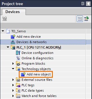
A “Add new object” window will open. In the Motion control tab, select the object “TO_PositioningAxis”, give it a name and click on “OK”.
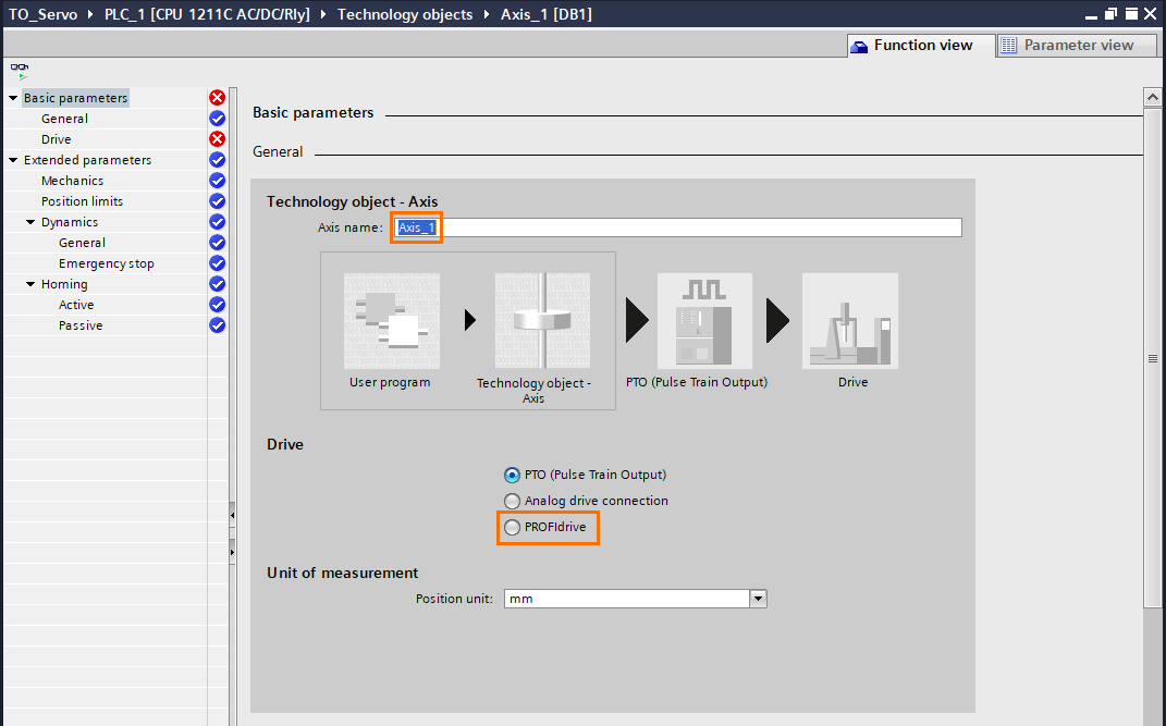
The TO_PositioningAxis is an object that simulates a mechanical axis. After configuring it with appropriate mechanical parameters, you will be able to execute positioning actions just by giving a position setpoint.
After creating the object, the parameters window of the TO will automatically open. In the basic parameters select “Profidrive” as a communication meaning.
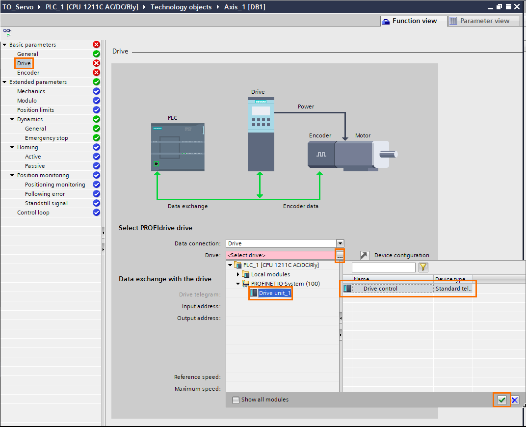
Next, click on the “Drive” tab. In the “Select Profidrive drive” section, click on the button with “...”, and select “Drive unit_1” then “Drive control”. Confirm by clicking on the green mark below.
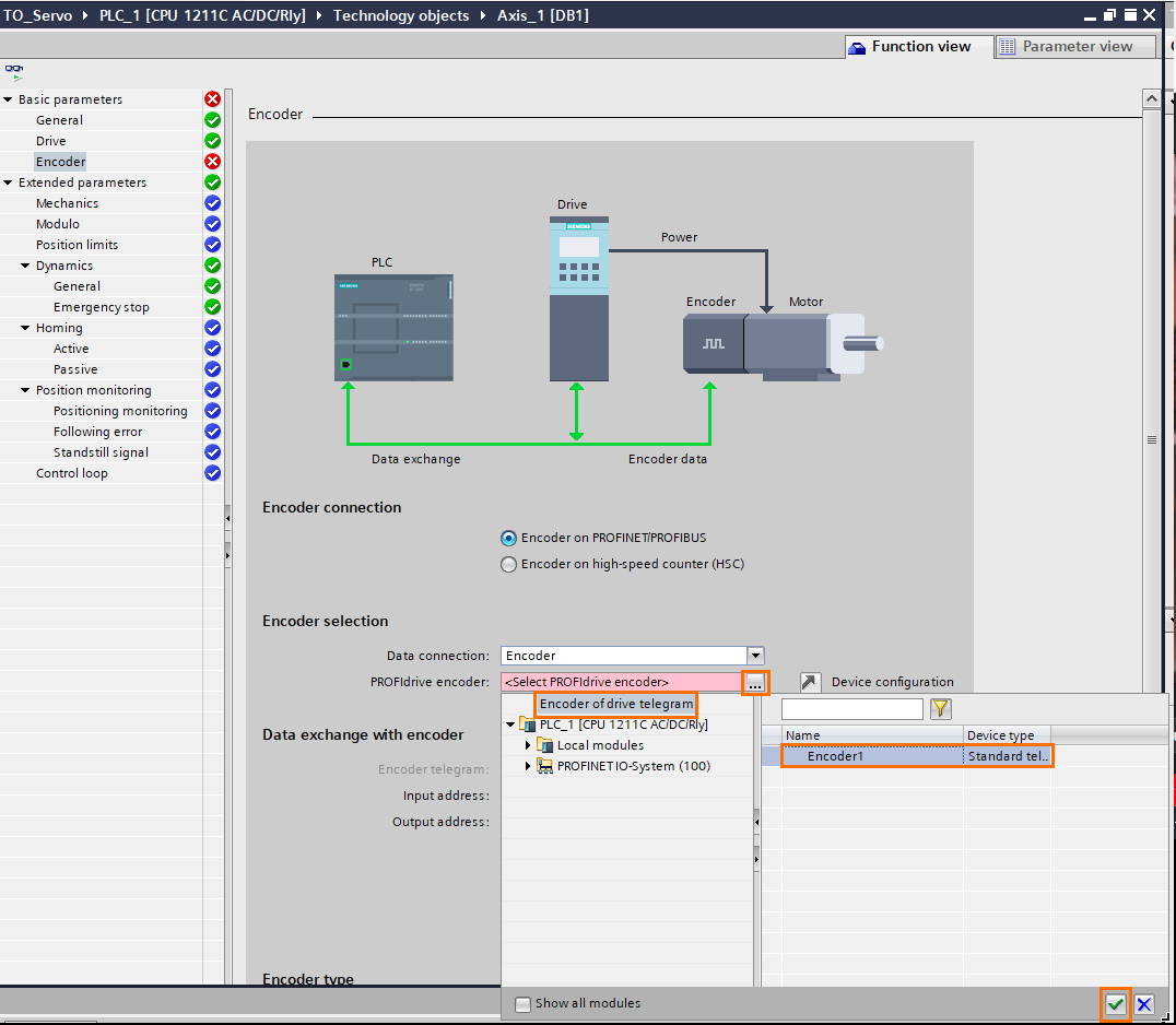
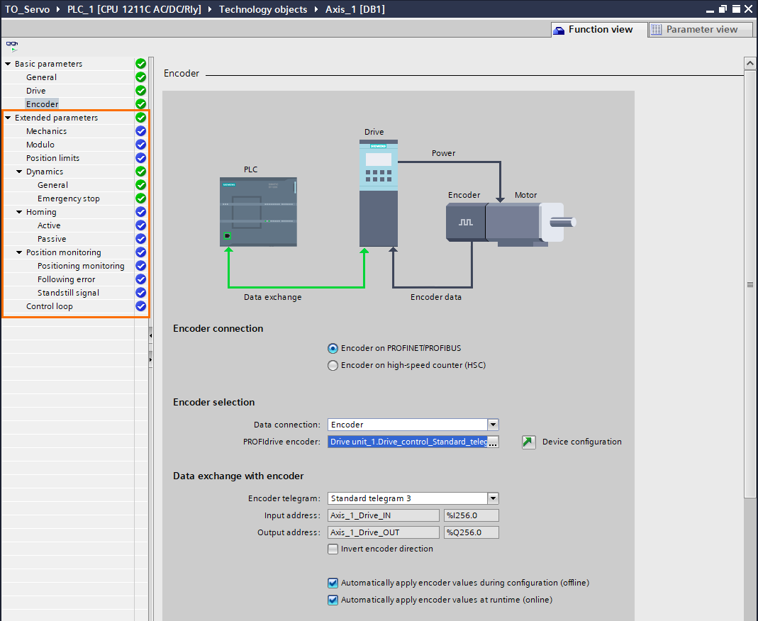
Next step, click on the “Encoder” tab, In the Encoder section, click on the “...” button, select “Encoder of drive telegram” then ‘Drive control’. Confirm with the green mark. This tells that the servo’s encoder is connected to the drive and its data will be sent through PROFINET
In the extended parameters you can set all the other parameters of your axis:
Type of motion (rotary or linear), motion directions, modulo, position limits (both software and physical using sensors), homing …etc
The values have been kept to their default values. Namely a simple rotary axis with a 1 for 1 coupling.
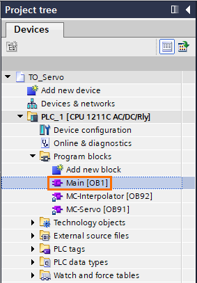
Now, to the programming. Open the “Program blocks” and click on “Main [OB1]”
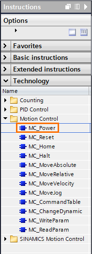
On the right side, in the “Instructions” section, Open the “Technology” section, then Open the “Moton control” folder and drag and drop an “MC_Power” instruction in Network 1.
A “Call options” will open. give a name to the block and click “OK”
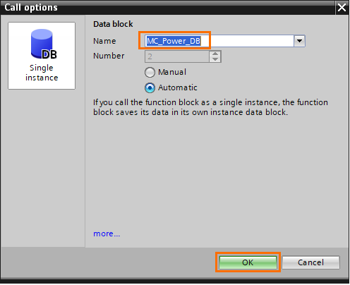
NB: This window will show each time you’ll create a new Motion Control instruction.
- The MC_Power is the instruction that enables the drive linked to it. This instruction must ALWAYS be present in your program. Otherwise, you won’t be able to operate the drive.
Edit the parameters of the instruction as follows.
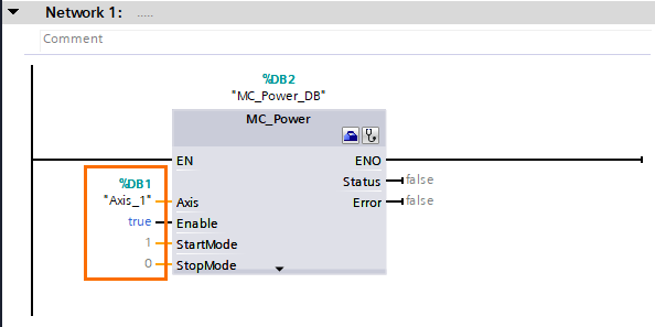
- The axis parameter must contain the Technology Object we created (Axis_1).
- The Enable parameter must contain a boolean. It could be any memory bit or set to TRUE or FALSE. In our case, it is set to TRUE so the drive will always be enabled.
- The StartMode and StopMode are parameters that define the behavior of the instruction during certain conditions such as alarms or failures. You can keep them at their default value.
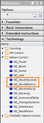
To control the servo motor, we will use the two most common instructions:
- MC_MoveAbsolute: orders the servo the move to an absolute position on the axis. The servo’s home is position 0.
- MC_MoveRelative: orders the servo to move to a position relative to its actual position.
Drag and drop MC_MoveAbsolute in Network 2 and fill the parameters as follows.
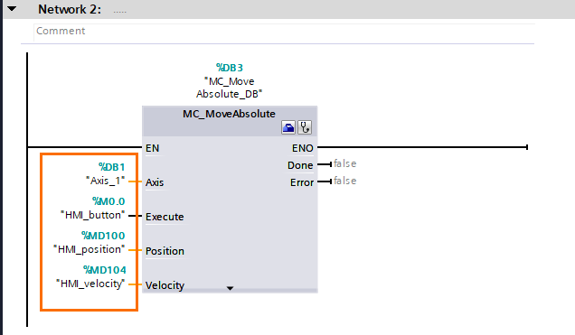
- The Axis parameter must contain the TO (Axis_1).
- The Execute parameter must contain bit memory that will trigger the instruction (For example, an HMI button).
- The Position and Velocity parameters are setpoint integers (For example, they can be set in an HMI).
Next, drag and drop MC_MoveRelative in Network 3 and fill the parameters as follows.
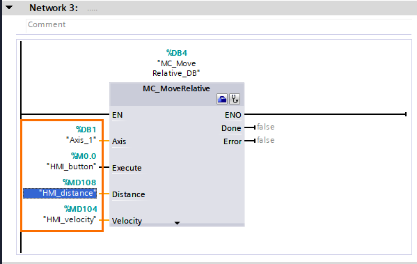
The parameters of this instruction follow the same logic as the previous one. The only difference is that MC_MoveAbsolute moves to a certain fixed Position while MC_MoveRelative travels a distance starting from its actual point.
Conclusion
In this tutorial, you learned how to configure a PROFINET configuration between a PLC and a servo drive, how to create a motion control Technology Object and how to simply execute basic positioning instructions.
As you can see, Siemens offers many powerful tools such as TOs which allow users to drastically reduce the development time, complexity, and harshness. Making it one of the best industrial environments to work with.
