An Introduction to Basic Ladder Logic Instructions in Siemens Tia Portal

Introduction

Siemens offers one of the most intuitive and user-friendly development environments. This makes it a great starting point for those who want to start practicing PLC programming. 

In this tutorial, we will explore the basic instructions available in the Siemens environment (defined by the IEC 61131-3 standard) by programming a simple box sorting machine in LADDER in TIA Portal. The purpose is to show how these instructions can be used in a real application.

Prerequisites

To follow along with this tutorial, you will need an installation of TIA Portal. We will be using TIA Portal v17, but you can use any other version.

No other hardware or software is required. 

Defining the specifications of the box sorting machine

The machine we’re building is a system where small and large boxes are fed in the entry of the machine and sorted by size (we assume only two kinds of boxes: larges and smalls). 

It is equipped with two push buttons (one for starting the machine and the other for stoping it) and two PhotoElectric (PE) digital sensors. One sensor is placed above the other to detect whether it’s a large or small box that’s entering (large boxes are taller than the small ones). Large boxes continue straight to the large box accumulator via Conveyor A while small ones are pushed (with a pneumatic cylinder controlled by a solenoid valve) towards Conveyor B which leads to a small box accumulator. Each conveyor is actuated by its motor at a constant speed.

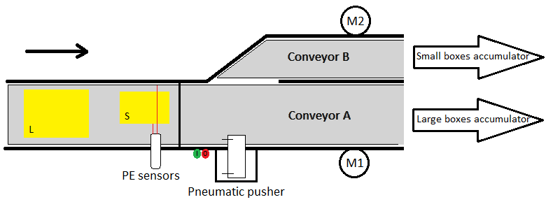
This machine must respect the following specifications.

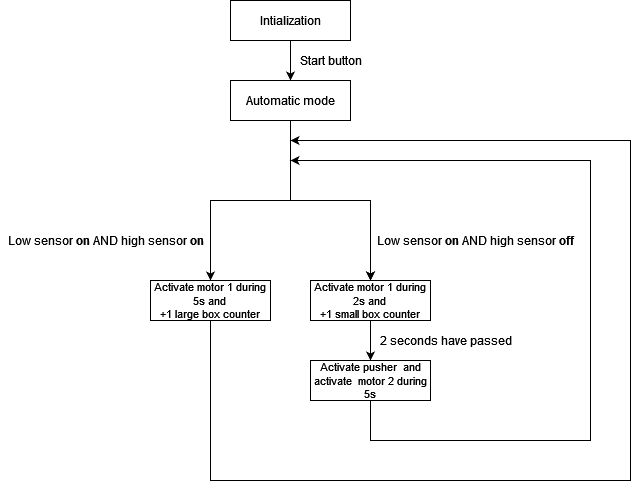
• If a small box enters: only the low sensor must turn on. The travel time from the position of the sensors to the large box accumulator is 5 seconds.
• If a large box enters, both sensors must turn on. The travel time from the sensors to the pneumatic cylinder is 2 seconds then the one from Conveyor B to the small box accumulator is 5 seconds.
• Counting the number of small/large boxes and their total.
• Calculate the percentage of small/large boxes.
• The machine must stop once at 1000 boxes.
  

The following chart summarizes the machines working.

We assume that all parts are wired as shown in the next two figures.

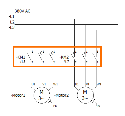
Both motors are asynchronous triphased motors. Each one is controlled by a contactor (KM1 and KM2).

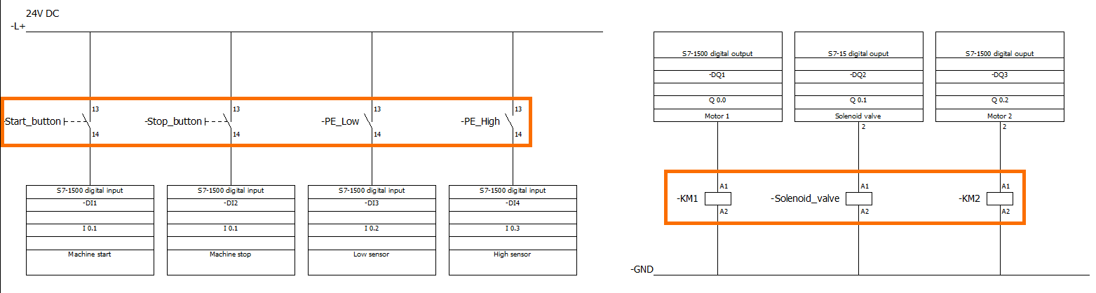
The start button, stop button, and both sensors (PE_Low and PE_High) are wired to 4 PLC digital inputs (from I 0.0 to I 0.3). The two contractors (KM1 and KM2) and the solenoid valve coils are wired to 3 PLC digital outputs (from Q 0.0 to Q 0.2).

Creating a new project in TIA Portal

Now that we have defined all the machine’s specifications, we can start writing our PLC program.

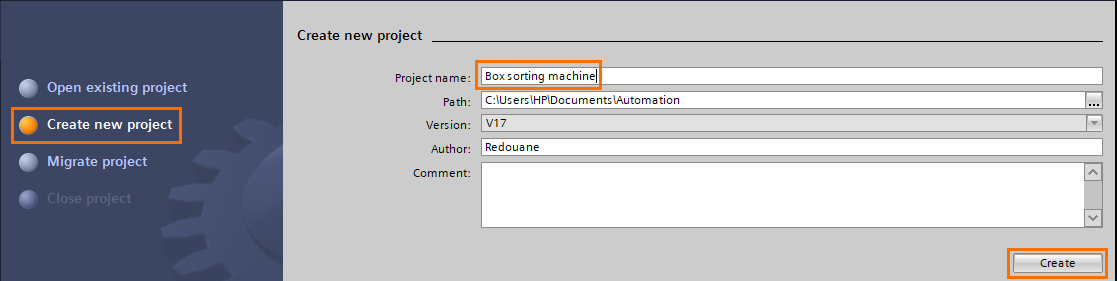
Start by launching TIA Portal. Then, on the first screen, click on “Create a new project”, give it a name (“Box sorting machine” in this instance), and click on “Create”.

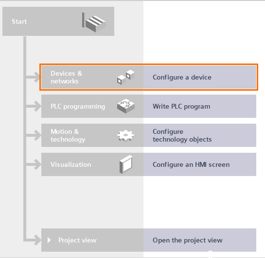
Then, on the next view click on “Configure a device”.

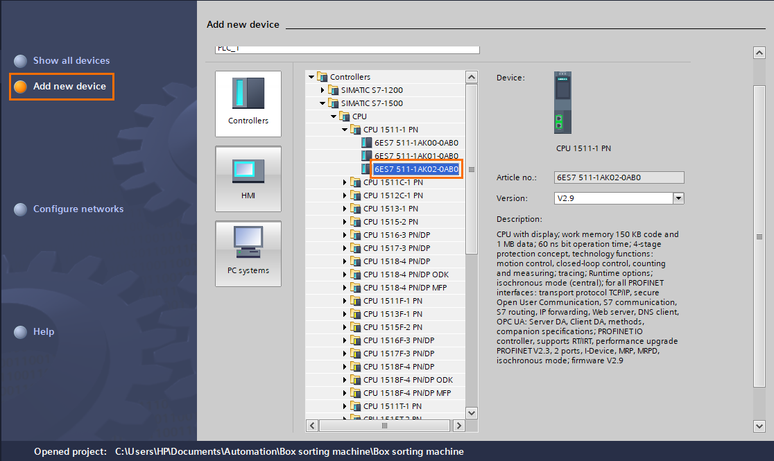
Once on the device configuration, click on “Add a new device”, open the folders “Controllers -> SIMATIC S7-1500 -> CPU -> CPU 1511-1 PN”, and select the 6ES7 511-1AK02-0AB0 CPU. 

Choosing this CPU specifically is not mandatory, you are free to choose the CPU you want. We simply selected the latest version of the simplest S7-1500 CPU.

Let the software initiate the project until the project’s interface appears.

Open the “Program blocks” folder on the Project tree then double click on “Main [OB1]”

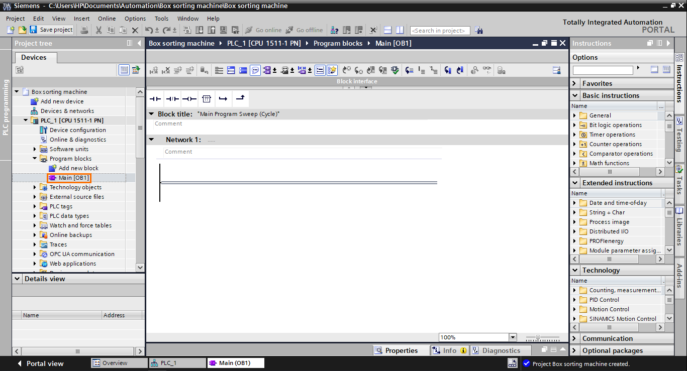
This is the main block of the project (OB1 for Organization Block 1). This is a cyclic block which means that all instructions that are programmed inside will be executed repetitively as long as the CPU is in RUN mode. We will program using only this block for more simplicity.

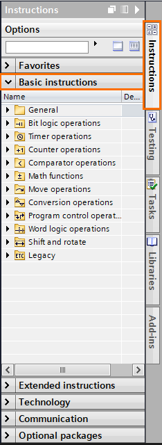
On the right side of the screen, you can find the instructions list. This can be accessed any time by clicking on the “Instructions” side tab. 

In this tutorial, we will be focusing only on the basic instructions. They contain all the tools we need to satisfy all the requirements we set.

Programming bit logic operations in TIA Portal

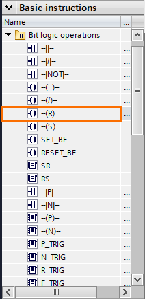
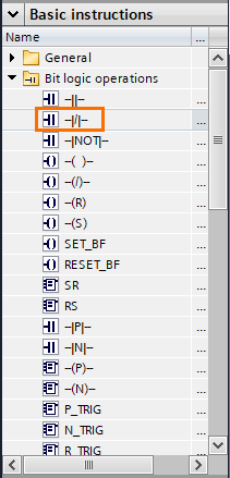
Open the “Bit Logic Operations” folder then drag and drop a normally open contact and a Set instruction on the line of Network 1.

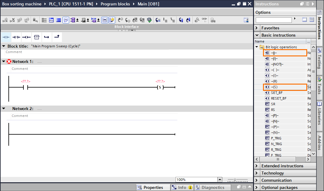
• The normally open contact is a bit interrogation. By adding this instruction, we are asking the state of the associated bit. If its state is 1, the program proceeds to execute the rest of the line. If its state is 0, the instructions after will not be executed 
• The Set instruction changes the state of a bit to 1. It stays at 1 as long as no other instruction changes its state.
  

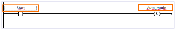
Now we have to associate a bit address to each instruction. First thing is to give it a tag. Click on the red question marks above the instructions and write the name as shown in the next figure.

As you can see, there’s a red line under our tags. This is normal because we didn’t define these tags yet. It can be done by right-clicking on the tag then clicking on “Define tag”.

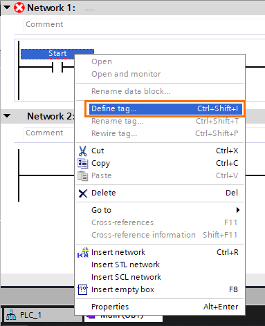
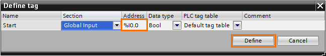
A small window will open asking you to define the data section, data type, and memory address of the tag. Define it as a Global input BOOL. Once done, the first physical address available will be automatically attributed to this tag. In our case, it is “%I0.0”. Once done, click on “Define”.

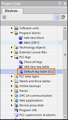
NB: You can access the list of all your tags at any time by opening the “PLC tags” folder in the Project tree and double-clicking on “Default tag table”.

Repeat the same actions to define the “auto_mode” tag. Define it as Global memory.

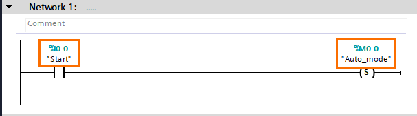
As you can see, there’s no longer a red line under our tags and the right memory address is shown above them. 

With these instructions, any time we press the Start button, the state of the memory bit “Auto_mode” will be set to 1. We will use the state of the “Auto_mode” bit as a condition to allow the functions we’ll program to be executed.

Now we need to add instructions that will change the state of “Auto_mode” to 0 when we press the stop button. To do so, drag and drop a normally open contact and a Reset Instruction to the Network 2.

Define the “Stop” tag for the NO contact as a Global input BOOL (its address will be automatically set to “I 0.1”) and assign “Auto_mode” to the Reset instruction.

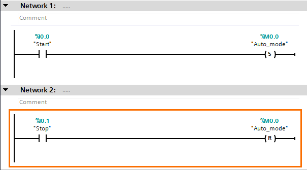
• The reset instruction changes the state of its associated bit to 0. As for the Set instruction, its state will stay at 0 until we change it with another instruction.
  

Now with Network 2, each time we press the stop button, the “Auto_mode” bit will be set to 0. 

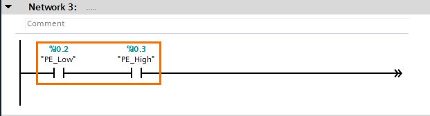
We are done with the buttons, it’s time to program the sensors. As we said earlier, the condition to detect a large box is having both sensors turned on. And the condition to detect a small box is having only the low sensor turned on and the high turned off. Let’s start by adding two NO contacts in Network 3, naming them “PE_Low” and “PE_High”, and defining their tags as Global input BOOL.

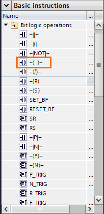
After this, add an assignment instruction right after the contacts. You can the assignment instruction in the “Bit logic operations” folder.

Drag and drop the instruction, name it “Large_box” and define it as a Local temp BOOL. 

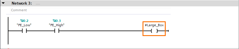
• The assignment instruction copies the logic state of the previous instructions executed before. If the previous logic result is 1, the associated bit will be set to 1. If the previous logic result is 0, the associated bit will be set to 0. 
  

This way, each time both sensors are at 1, the “Large_Box” will be set 1. Telling us that a large box just passed through the sensors.

Let’s do the same but for small boxes. Repeat the same actions we just did but use a normally close contact for “PE_High”. You can find the normally closed contact in the “Bit logic operations” folder.

Use the “Small_box” tag name for the assignment instruction.

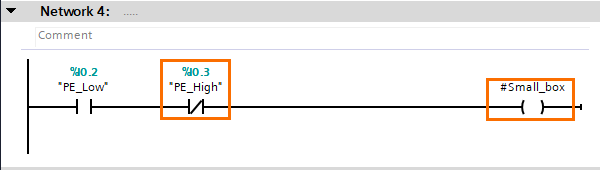
• The normally closed contact is a bit interrogation. By adding this instruction, we are asking the state of the associated bit. If its state is 0, the program proceeds to execute the rest of the line. If its state is 1, the instructions after will not be executed.
  

In this case, the “Small_box” bit will be set to 1 only if “PE_Low” is at 1 and “PE_High” is at 0.

Programming timers in TIA Portal

Okay, we defined all the conditions bits we need. Now let’s start programming the behavior of the pusher and motors. Since the specifications require a time-based control, we will use timers to activate them.

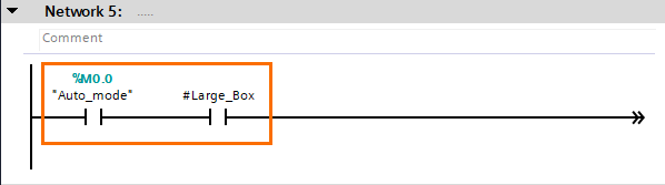
First, we will define the conveyor’s A behavior (large boxes). add two normally open contacts to Network 4. And define them as “Auto_mode” and “Large_box”.

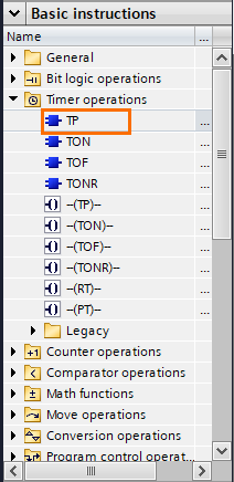
From the “Timer operations” folder, drag and drop a TP instruction.

Upon dropping the instruction, a “Call options” window will open, asking you to create a DB (Data Block) that will contain all the timer’s information. Simply name the DB “timerA_DB” and click on OK.

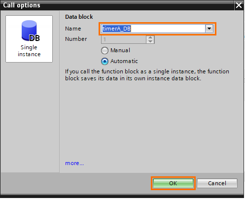
NB: This window will open each time you’ll create a timer or a counter. Let the DB’s number be set automatically.

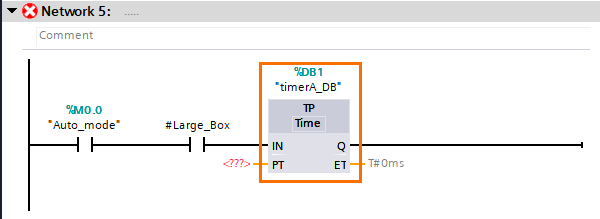
• The TP timer is a pulse timer instruction. It is activated by receiving a 1 at the IN input and sets the output Q at 1 during an amount of time specified in the PT input and returns the current time in the ET output. If the IN input is set to 1 multiple time while the counter is active, it does not affect the current time value.
  

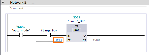
The PT input requires a TIME data type. To define a TIME data, you have to write “T#” then specify a time duration with its unit. For this case, we want the timer to run for 5 seconds. So we have to write “T#5s”.

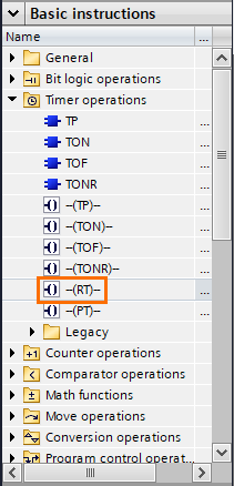
If the instruction is kept like that, it’ll cause a malfunction in the machine. Since resetting the input does not reset the current time, this means that if multiple large boxes pass within 5 seconds, the Q output will be set to 1 for 5 seconds once only. To avoid that, we just have to add a “Reset timer” instruction just before the IN input. You can find the “Reset timer” instruction in the “Timer operations 

Assign the reset timer function to “timerA_DB”.

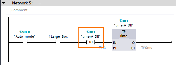
This way, any time the IN input would be set to 1, it will reset the timer just before. 

NB: This logic will be applied for all other timers used in the rest of this tutorial.

Now we just have to add an assignment instruction right after the Q output. Name it “Motor1” and define it as a Global output BOOL.

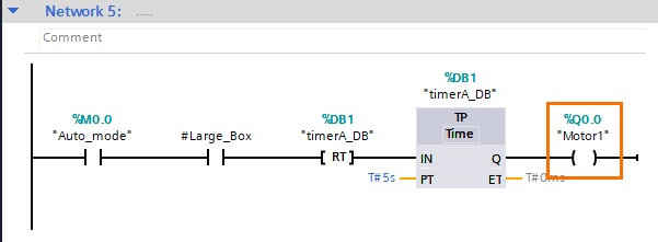
Great, now motor 1 will be turned on following our specifications.

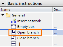
Let’s build the machine’s behavior for small boxes. Since we already have an “Auto_mode” bit interrogation, no need to add another one. We can simply add a new branch right after the interrogation. You can find the open branch instruction in the “General” folder.

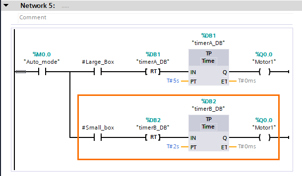
In this new branch, we will build the first step of conveyor B behavior. Which is turning on conveyor A for 2 seconds (moving the box from the sensors to the pusher’s position). Name the timer “timerB_DB” and define the assignment instruction as “Motor1”. 

Let’s do the second step which is activating the solenoid valve after 2 seconds have passed. To do this, we’ll add another branch right after the “Large_box” integration and this time, we’ll use a TON timer (found in the “Timer operations” folder). Name the timer “timerC_DB”, Set PT at 2 seconds, and define “Solenoid_valve” as a Global output BOOL.

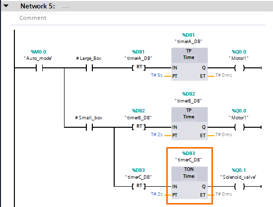
• The TON timer is an on-delay timer instruction. It is activated by receiving a 1 at the IN input and sets the output Q at 1 after the amount of time specified in the PT input has passed and returns the current time in the ET output. If the IN input is set to 1 multiple time while the counter is active, it does not affect the current time value.
  

With this timer, the solenoid valve is going to be activated after 2 seconds passed since the sensors detected the small box. 

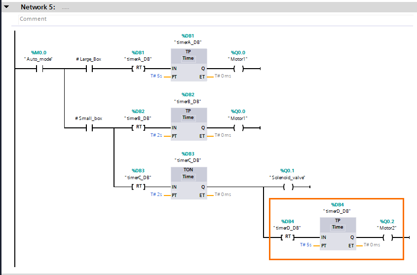
For the third step, we need motor 2 to be activated for 5 seconds at the same time as the activation of the pusher. Add a new branch right after the output of “timerC_DB”. Then add a simple TP timer (with its reset), name it “timerD_DB”, and set it at 5 seconds. Right after, add an assignment instruction, name it “Motor2” and define it as a Global output BOOL.

Programming counters in TIA Portal

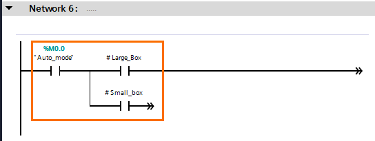
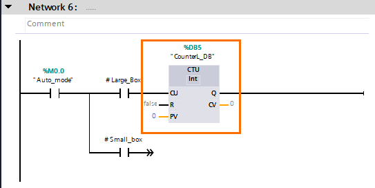
Now with the machine’s behavior achieved, let’s add counters to measure the number of large and small boxes. First, add an “Auto_mode” NO contact followed by two branches: one leading to a “Large_box” NO contact and the other to a “Small_box” NO contact in Network 6 as shown in the next figure.

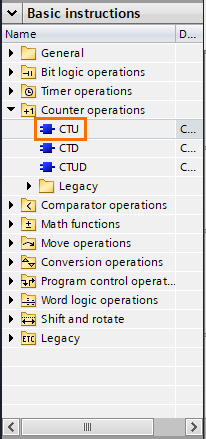
Right after the “Large_box” contact, add a CTU (CounterUp) instruction and name it “CounterL_DB” (in the call options window). You can find it in the “counter operations” folder.

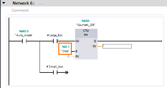
• The CTU instruction counts the number of times the CU input is set to 1. It starts counting from the value in the PV input and returns the actual counter value in the CV output. You can reset the counter to its first value by setting a 1 in the R input.
  

Let the PV input at 0 (as a constant) and assign the “Stop” bit to the  R input.

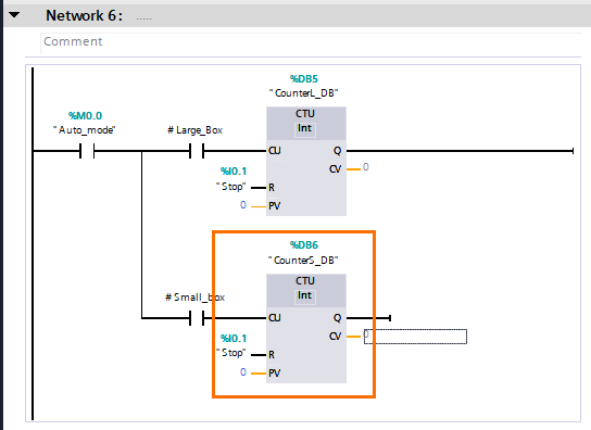
Go ahead and repeat the same step for the counter after the “Small_box” contact.

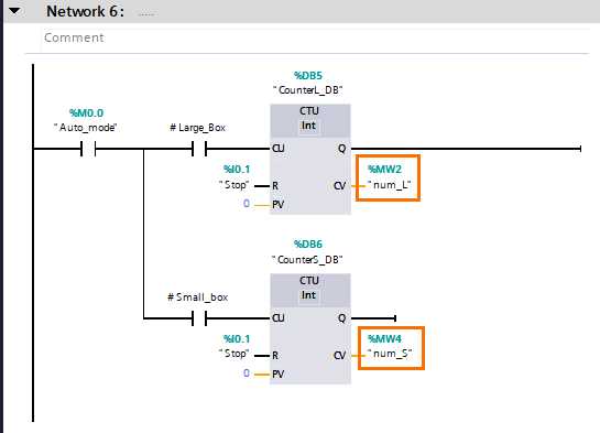
To retrieve the current counter values, we have to assign integer tags to the CV outputs. Define the two tags “num_L” and “num_S” as Global memory INTs as shown in the next figure.

Programming math and conversion instructions in TIA Portal

In this part of the tutorial, we’re gonna take the counter values we just programmed and do some math with them to calculate: the total number of boxes and the percentage of large/small boxes.

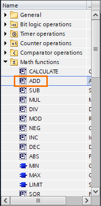
First, we will calculate the total number of boxes which is the sum of the number of large and small boxes. To do this, add an “Auto_mode” NO contact to Network 7 followed by an ADD instruction. You can find it in the “Math functions” folder. 

Assign “num_L” to IN1 and “num_S” to IN2 then define “total_box” as a Global memory INT to OUT.

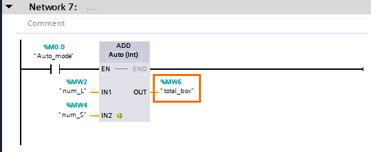
• The ADD instruction sums the numerical values in IN1 and IN2 inputs and returns the result in the OUT output. The summed inputs and the output result have the same data type.
  

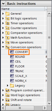
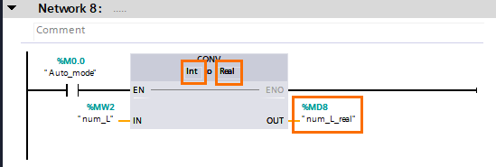
Now let’s calculate the percentages of large and small boxes. To do so, we must first convert “num_L”, “num_S” and “total_box” from INTs to REALs. To do this, add an “Auto_mode” NO contact followed by a CONVERT instruction to Network 8. You can find it in the “Conversion operations” folder. 

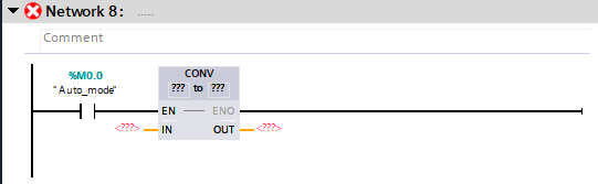
• The CONVERT instruction converts the data type set in the IN input to another data type returned in the OUT output. The nature of the conversion is determined by the “??? to ???” slots (For example INT to REAL).
  

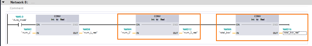
Set the conversion to be an “INT to REAL”, assign “num_L” to the IN input, and define “num_L_real” as a Global memory Real.

Go ahead and repeat the same steps for “num_S” and “total_box”.

To calculate the large boxes percentage, we have to divide the number of large boxes by the number of the total number of boxes then multiply the result by 100.

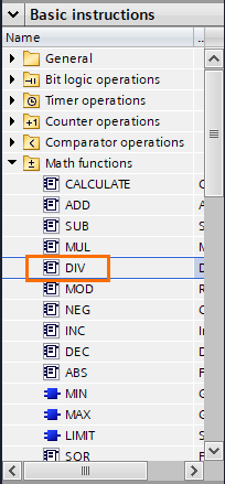
Add an “Auto_mode” NO contact in Network 9 followed by a DIV (Divide) instruction. You can find it in the “Math functions” folder.

Define “division” as a Local temp REAL and make sure that the type of division is recognized as real.

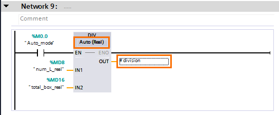
• The DIV instruction divides the value in IN1 by the value in IN2 and returns the result in OUT. IN1, IN2, and OUT have the same data type and it is set by the DIV type slot.
  

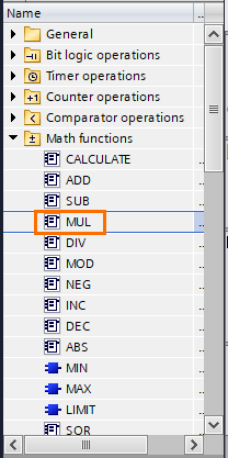
Now we have to multiply the value in “division” by 100 to obtain a percentage. For this, add a MUL (Multiply) instruction. You can find it in the “Math functions” folder.

Assign the inputs and outputs as shown in the next figure.

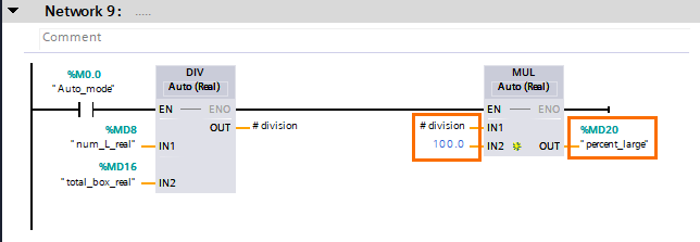
• The DIV instruction multiplies the value in IN1 by the value in IN2 and returns the result in OUT. IN1, IN2, and OUT have the same data type and it is set by the MUL type slot.
  

NB: You must write 100.0 instead of simply 100 for it to be recognized as a real number. Otherwise, it will take it as an integer.

Now that we calculated the percentage of large boxes “percent_large”, we can repeat these steps and calculate the percentage of small boxes. Or, we can simply subtract the percentage of large boxes from 100%. Since there are only two types of boxes, it is way easier to just do a subtraction. For this, add a SUB instruction (found in the “Math functions”) and define the inputs and output as shown in the next figure.

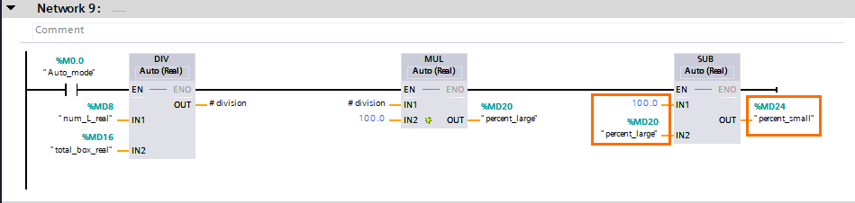
• The SUB instruction subtracts the value in IN2 from the value in IN1 and returns the result in the OUT output. IN1, IN2, and OUT have the same data type and it is set by the SUB type slot.
  

Programming comparison and move instructions in TIA Portal

In some cases, you’ll need to trigger events when a counter reaches a certain value. In our case, we want to stop the machine when the total number of boxes reaches 1000. 

We can achieve this by simply using an “Auto_mode” reset instruction preceded by a CMP == instruction. You can find it in the “Comparator operations” folder.

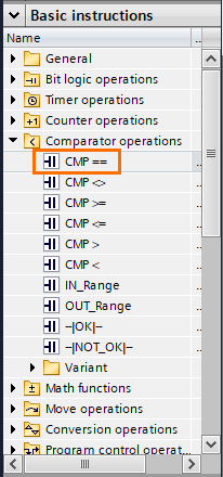
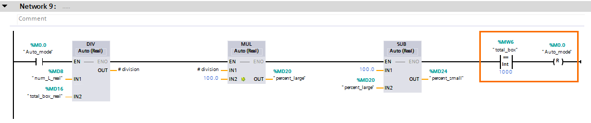
• The CMP instruction compares the upper value to the bottom one according to a certain condition (in our case, equality ==). If the condition is verified, the program proceeds to execute the rest of the line. If it’s not, the instructions after will not be executed. Both compared values must have the same data type.
  

Here, when the value of “total_box” equals 1000, the reset instruction activates and sets the value of “Auto_mode” to 0.

One last thing to conclude this tutorial is to reset to 0 the values of the reals we created once the machine is stopped to prevent a memory overlap on the next starting. To do this, we will use the MOVE instruction. 

Add an “Auto_mode” reset instruction preceded by a MOVE instruction in Network 10. You can find it in the “Move operations” folder.

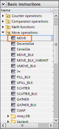
• The Move function copies the value from its input to its output. The input and the output must have the same data type.
  

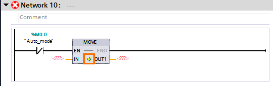
Click twice on the yellow star in the MOVE instruction to add two more outputs. and fill the tags as shown in the next figure.

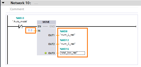
This way each time the machine is stopped, it will bring back the values of the reals to 0.

Conclusion

In this tutorial, you learned how to program, step-by-step, a simple machine using only basic instructions in TIA Portal. 

Siemens has gone to great lengths to make its development environment as enjoyable to use for beginners as it is for veterans. Thanks to the IEC 61131 standardization, all instructions that we have explored in this tutorial will be similar in other development environments such as RSLogix 5000.

As an exercise, you could try to reproduce this project using other environments from other PLC manufacturers to fully discover all the subtle differences between them.