How To Program PID Loops In RSLogix 500

Introduction 

In this tutorial, we are going to cover what a PID loop is, take a look at some of the typical uses, and finally run through an introduction of how to implement a PID loop in RSLogix 500.

What is a PID Loop and How it Works

What is a PID loop? PID is an acronym for Proportional, Integral, Derivative. Also known as a 3 term controller because it has three terms, they are used to modulate an output known as a Control Variable (CV) based on a Process Variable (PV), in relation to a set point (SP). They are extremely popular because of their flexibility, their optimal performance for closed-loop systems, and the ease in which they can be turned on the fly by plant operators without them having to know extensively about controls engineering.

Let’s break it down and figure out what each term of the PID loop does, how it does it, and what to expect when it is adjusted.

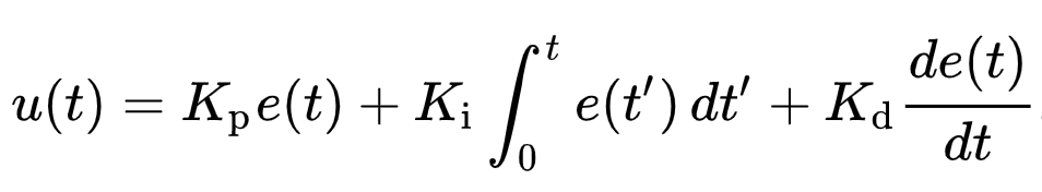
The important parts of this equation are Kp, Ki, and Kd. u(t) is the controller output, and e(t) is the error value.

Kp – Proportional Gain

Increasing the proportional gain, Kp, has the effect of proportionally increasing the control signal for the same level of error. This makes the controller react quicker for a given error in the closed-loop system, but it also means that it will likely overshoot more as well.

Increasing Kp also tends to reduce, but not eliminate, the steady-state error. The steady-state error is the difference between the input and the output of a system as time goes to infinity. This is another way of saying that the response has reached a steady state.

Ki – Integral Gain

The addition of an integral term to the controller, Ki, helps to reduce the steady-state error. If there is a persistent, steady error, the integrator builds over time, increasing the control signal and driving the error down. This has the adverse effect of making a system sluggish and oscillatory since when the error signal changes sign, it may take a while for the integrator to unwind, leading to an overshoot in the opposite direction.

Kd – Differential Gain

The addition of a derivative term to the controller, Kd, adds the ability of the controller to anticipate an error. With simple proportional control, if Kp is fixed, the only way that the control will increase is if the error increases. With derivative control, the control signal can become large if the error begins sloping upward, even while the magnitude of the error is still relatively small. This anticipation tends to add damping to the system, thereby decreasing overshoot. The addition of a derivative term, however, has no effect on the steady-state error.

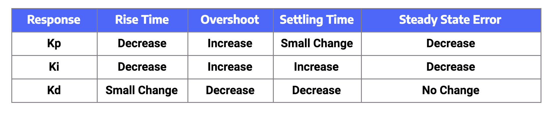
The table shows the general effects of each of the control parameters Kp, Ki, and Kd in a closed-loop system. Although these apply to most closed-loop systems, it is not a fit-for-all and some systems may respond differently.

The example graph demonstrates the response of a PID controller based on changing the parameters. This is an example only and these parameters will respond differently in different applications.

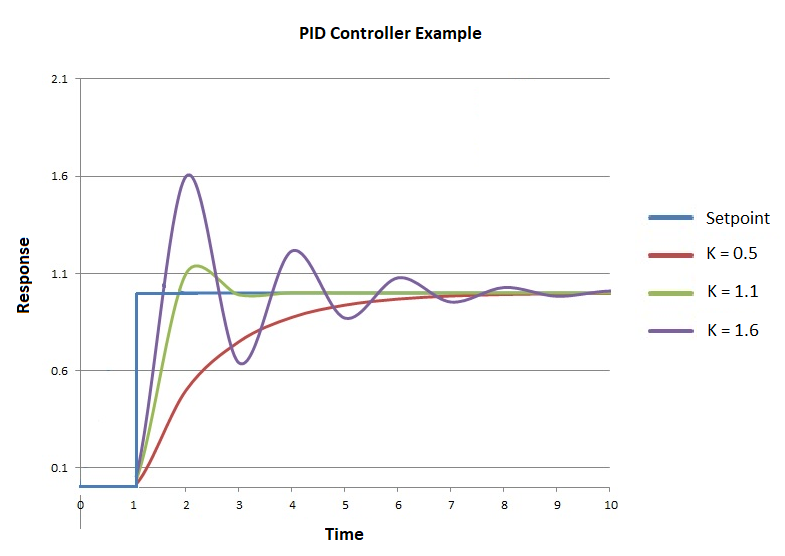
The controller with K = 0.5 reacts slowly and reaches the setpoint with no overshoot. This condition is referred to as overdamped. This response is very stable, but being so slow means it is usually not beneficial in most applications.

The controller with K = 1.6 reacts fast and severely overshoots the setpoint. The controller adjusts accordingly so that the output eventually settles down at the setpoint. This condition is referred to as underdamped. This response is very fast but has poor stability. It is usually not beneficial to have such an unstable response.

The controller with K = 1.1 reaches the setpoint quickly with minimal overshoot. The response is not as stable as K = 0.5, and not as quick as K = 1.6, but this type of response is usually most appropriate and a good compromise for most applications.

That being said, each PID controller application is different and they need to be tuned accordingly to gain the best outcome. Sometimes an overshoot is acceptable for a faster response, and sometimes the process is slow, so a slow response is best. The Kp, Ki, and Kd values need to be adjusted appropriately to achieve the desired response.

Tuning a PID Loop – Starting Values

When setting up a PID loop initially, what values should you use as a starting point? This is a good question, and there is no hard and fast rule. The Ziegler-Nichols Tuning method is considered a good method of tuning PID loops.

The Ziegler-Nichols rule is a heuristic PID tuning rule that attempts to produce good values for the three PID gain parameters by doing the following;

1. Set all gains to zero (0)
2. Increase Proportional gain until the response is a steady sine wave oscillation
3. Increase the Derivative gain until the oscillations are stopped – this makes it critically damped
4. Repeat steps 2 and 3 until the Derivative gain does not stop the oscillations
5. Set Proportional and Derivative gains to last stable values
6. Increase the Integral gain until you reach the setpoint with a desired number of oscillations. Remember overshooting is not always a bad thing, it means it will achieve the setpoint quicker.
   

This is just one method of tuning a PID Loop, but whatever method you use, finding the right balance for the application it is used in is always key.

Using all of this, how can we apply this into RSLogix 500 and create our own PID loops for plant control?

Well, in RSLogix 500, we have a lot of parameters to input to begin with, but the main ones are the same, Kp, Ki, and Kd.

It is important to point out that in RSLogix 500, Kp is referred to as Kc, Ki is referred to as Ti, and Kd is referred to as Td. From this point onwards, that is what we shall also refer to them as.

Parameterising a PID in RSLogix 500

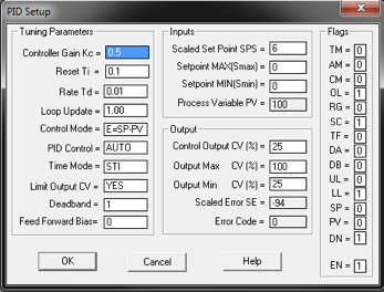
We’ve already covered the main inputs Kc, Ti, and Td, so we’ll look at some of the other important parameters.

Loop update – This is the time interval between PID calculations. The entry is in 0.01 second intervals. Generally, enter a loop update time five to ten times faster than the natural period of the load.

Control Mode – Select either E = SP – PV (Reverse Acting) or E = PV – SP (Direct Acting).

Reverse acting causes the output CV to increase when the input PV is smaller than the setpoint SP (for example, a heating application). Direct acting causes the output CV to increase when the input PV is larger than the setpoint SP (for example, a cooling application).

Deadband DB – Value from 0 to the scaled maximum, or 0-16383 when no scaling exists.

This deadband extends above and below the setpoint by the value you enter. The deadband is entered at the zero crossing of the process variable PV and the setpoint SP. This means that the deadband is in effect only after the process variable PV enters the deadband and passes through the setpoint. Once the process variable PV is within the deadband (setpoint +/- Deadband DB) then the output of the PID controller does not increase or decrease. When the process variable PV moves outside of the deadband, the output value once again begins to modulate.

Limit Output CV – Select Yes or No. Selecting Yes limits the output to minimum and maximum values. Selecting No applies no limits to the output.

Control Output CV (%) – in manual mode, a value from 0-16383 can be entered to output to the device. In auto mode, the output to the device is calculated by the PID controller.

Output Min (CV%) – If Limit Output CV is Yes, the value you enter is the minimum output percent that the control variable CV will obtain. If CV drops below this minimum value, the CV is set to the value you entered and the output alarm lower limit (LL) bit is set. If the limit Output CV is No, the value you enter determines when the output alarm lower limit bit is set. If CV drops below this minimum value, the output alarm lower limit (LL) bit is set. An example of where limiting the loop to a minimum value is useful is for a pump that is required to run above a certain speed.

Output Max (CV%) – If Limit Output CV is Yes, the value you enter is the maximum output percent that the control variable CV will obtain. If CV exceeds this maximum, the CV is set to the value you entered, and the output alarm, upper limit (UL) bit is set. If the limit Output CV is No, the value you enter determines when the output alarm upper limit bit is set. If CV exceeds this maximum value, the output alarm, upper limit (UL) bit is set.

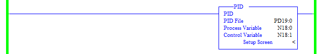
In the above Figure 1, you can see that the PID file is defined as PD19:0. This sets up all the parameters needed for the PID block which is accessible within the whole project.

The above Figure 2 is where the parameters can be set up. Alternatively, these can be hardcoded. See figure

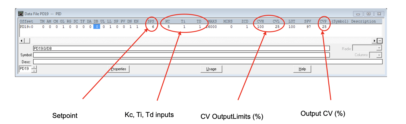
The above Figure 3 shows the PD19 Data file with all of the elements that make up the PID loop controller. Highlighted are some of the parameter elements discussed earlier in the tutorial.

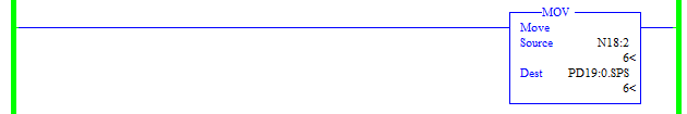
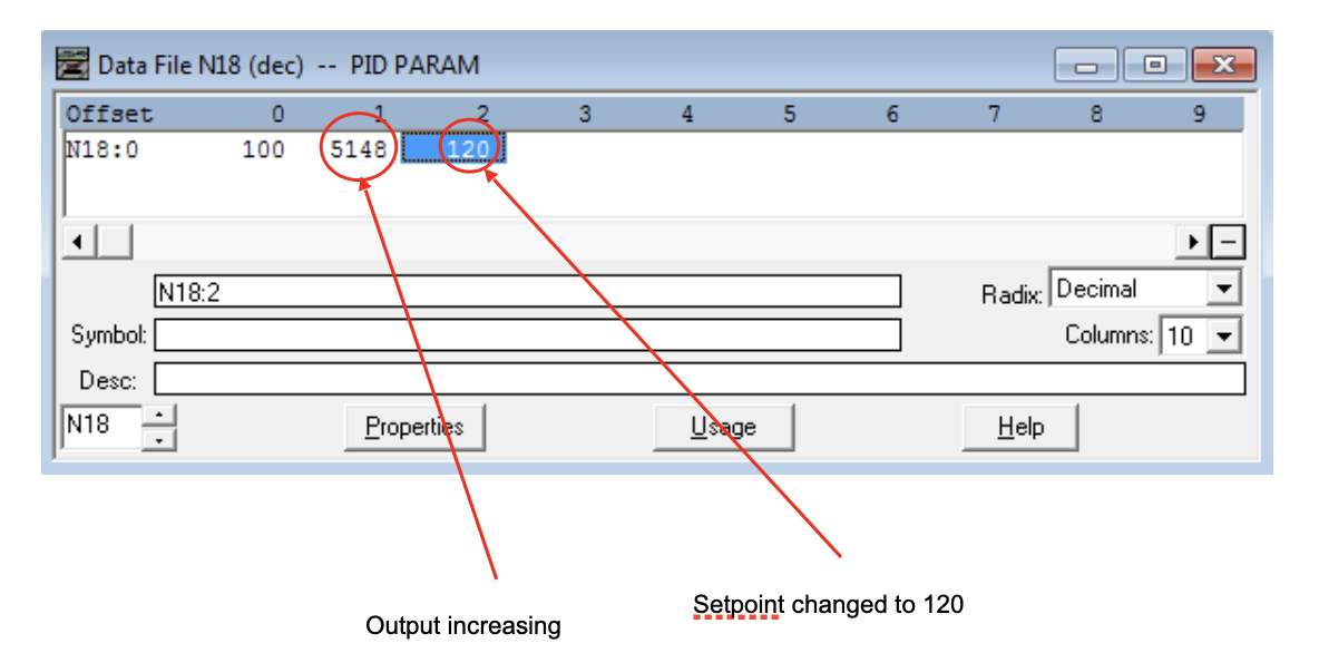
In the above Figure 4, you can assign a value to one of the PID parameters by using a MOV instruction to move the desired value to the appropriate PID parameter, in this case to the PID setpoint. In the case of N18:2, this could be a value from an HMI or SCADA display to allow an operator to increase or decrease the setpoint to adjust the desired output.

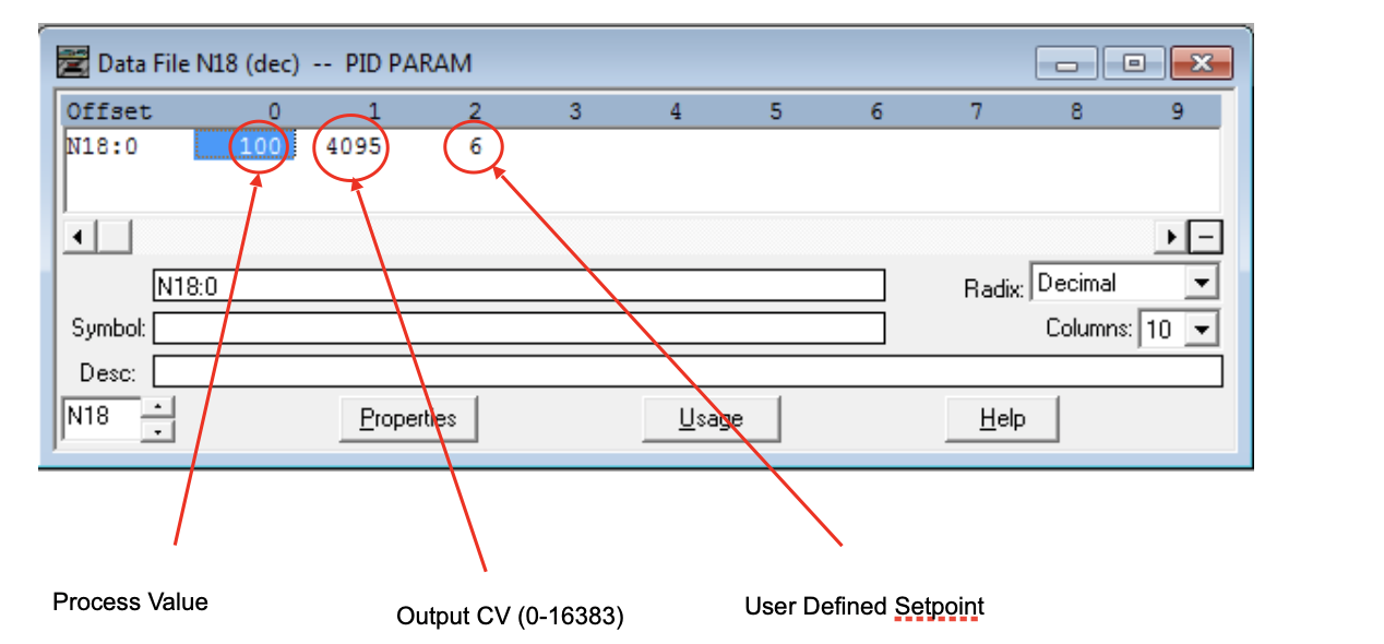
The above Figure 5 displays the Data file for N18.

N18:0 is used as per Figure 1 for the PID Process Variable (PV).

N18:1 is the Control Variable (CV) Output.

N18:2 is as above in Figure 4, to assign a setpoint parameter.

In this example, the Setpoint is below the Process Value, so the Output Control Value is reduced towards 0. Figure 3 shows that the Output Min CV is set to 25% (16383 = 100%, so (16383/100)*25 = 4095). If we change the setpoint value to a value greater than 100, let’s use 120 like in Figure 6 below, we see the Output Control Variable value increase.

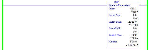
By scaling the Output Control Variable to a percentage, we can determine, for example, how much the output is opening a valve or the speed of a Variable Speed Drive (VSD). As detailed earlier in the tutorial, the Output Control Variable is in the range 0-16383. Scaling this as above in Figure 7 between scaled Min and Max values of 0 and 100 respectively gives us the full working range of the output 0 -100 %

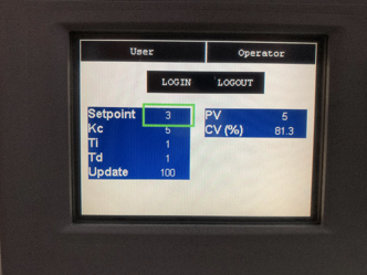
As you can see from Figure 8 above, the input variables are set via an HMI interface. In this example, the CV value is decreasing because the Process Value PV (5) is greater than the Setpoint value (3). The Control Value is displayed as a percentage (%).

Conclusion

That’s it for this tutorial, I hope you’ve learned something about PID loops, and how to configure them in RSLogix 500. They are a very useful and versatile tool to use in software programming and are used everywhere, from controlling temperature devices with temperature control valves to controlling the speed of a Variable Speed Drive based on airflow. There is really no right and wrong way to tune a PID loop. Sometimes you want a really fast response and don’t really mind if it overshoots. Sometimes it is critical for no overshoots, and the time it takes isn’t an issue. There is no one size fits all, and each application is different. Finding the right balance is what matters!